


By Conor McCarthy
As part of KX25, the international kdb+ user conference held May 18th in New York City, a series of seven Juypter notebooks were released and are now available on https://code.staging.kx.com/q/ml/. Each notebook demonstrates how to implement a different machine learning technique in kdb+, primarily using embedPy, to solve all kinds of machine learning problems, from feature extraction to fitting and testing a model. These notebooks act as a foundation to our users, allowing them to manipulate the code and get access to the exciting world of machine learning within KX. (For more about the KX machine learning team please watch Andrew Wilson’s presentation at KX25 on the KX Youtube channel).
The open source notebook outlined in this blog, describes the use of a common machine learning technique called decision trees. We focus here on a decision tree which provides an ability to classify if a cancerous tumor is malignant or benign. The notebook shows the use of both q and Python to leverage the areas where they respectively provide advantages in data manipulation and visualization.
Background
Decision trees are a simple yet effective algorithm used primarily in supervised classification and regression problems. The goal of such an algorithm is to predict the value of a target variable based on several input variables. To do this, data is split based on the value of a binary feature (Age < 20, Height > 6ft etc.). Splits occur at interior nodes associated with the input variables in the data set and splitting of this form continues until a desired depth is reached. The task of such models is thus to fit a decision tree to the data by finding the sequence of splits and optimal values which lead to the most accurate model.
Decision trees have a number of advantages as a method for machine learning:
- They can manage a mix of continuous, discrete and categorical data inputs.
- They do not require normalization or pre-processing.
- They produce outputs that can be easily interpreted and visualized
One of the main disadvantages of decision trees surrounds the creation of over-complex trees which are not easily generalized from the training data, this can arise if the depth of the tree has been set too high or the minimum number of leaves in a branch is set too low. Trees can also be non-robust with small changes in data having a large effect on the final results which also makes generalization difficult. These issues are improved through the implementation of a random forest algorithm which is a large collection of decision trees. This algorithm will be discussed in depth in the final blog of this series titled ‘Random Forests in KX’ to be released next week.
Technical Description
As mentioned above, this notebook provides an example of a model used for the classification of cancerous tumors. To do this scikit-learn is used to load the UCI Wisconsin Breast Cancer (Diagnostics) dataset, also used in the fourth blog in this series ‘Classification using K-Nearest Neighbors in kdb+.’ This data set contains information from 596 samples, each of which includes 30 distinct cell characteristics (texture, area, etc.) labeled as ‘data,’ and the classification of the tumors as malignant or benign which is labeled as the ‘target.’
Some initial analysis on the unprocessed data is completed showing the shape of the dataset and the distribution of benign to malignant tumors present within the dataset. The data is then split 50/50 into a training and test set using the q traintestsplit function from the func.q script available on GitHub.
We apply the ‘sklearn.tree’ package ‘DecisionTreeClassifier’ to the training set to fit the data at a maximum depth of three. This algorithm finds the best tree by finding a feature (mean concave points) and split value (0.052) which most effectively partitions the benign and malignant data. We can then, via embedPy, use graphviz to produce an easy to understand graphical representation of the fitted data as follows.
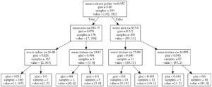
Looking at the data following the first split into subsets of 176 and 108 samples these individual sets contained the following number of malignant and benign tumors,
| No. Samples | Malignant | Benign |
| 176 | 7 (4%) | 169 (96%) |
| 108 | 95 (88%) | 13 (12%) |
As such, after just one split we can already see the predictive power of this model where the data has been partitioned into being mostly benign or malignant based on the mean number of concave points on the tumor. Following the complete training of this model we can evaluate both its accuracy and log loss by passing it the test data. Within this notebook the calculation of accuracy uses q via functions contained within the script func.q while log loss is calculated using q and Python.
Finally, both a confusion matrix (to find the number of true or false, positive or negatives results) and a receiver operating characteristic (ROC) curve used to find the relationship between the true positive rate (sensitivity) and false positive rate (specificity) are produced to provide a visual representation of the accuracy of our model.
If you would like to further investigate the uses of embedPy and machine learning algorithms in KX, check out the ML 05 Decision Trees notebook at (https://github.com/KxSystems/mlnotebooks), where several functions commonly employed in machine learning problems are also provided together with some functions to create several interesting graphics. You can use Anaconda to integrate into your Python installation to set up your machine learning environment, or you can build your own by downloading kdb+, embedPy and JupyterQ. You can find the installation steps on code.staging.kx.com/q/ml/setup/.
Don’t hesitate to contact ai@devweb.kx.com if you have any suggestions or queries.
Other articles in this JupyterQ series of blogs by the KX Machine Learning Team:
Natural Language Processing in kdb+ by Fionnuala Carr
Neural Networks in kdb+ by Esperanza López Aguilera
Dimensionality Reduction in kdb+ by Conor McCarthy
Classification Using k-Nearest Neighbors in kdb+ by Fionnuala Carr
Feature Engineering in kdb+ by Fionnuala Carr
Random Forests in kdb+ by Esperanza López Aguilera
References:
- Kotsiantis, S.B. Decision Trees: A Recent Overview. Artif Intell Rev (2013) 39: 261. Available at: https://doi.org/10.1007/s10462-011-9272-4
- Breiman, L., Friedman, J.H., Olsen, R.A., Stone, C.J., Classification and regression trees, Wadsworth, USA, 1984. Available at: https://rafalab.github.io/pages/649/section-11.pdf
- Quinlan, J.R., Induction of decision trees, Machine Learning, num. 1, pp. 81-106, 1986. Available at: http://hunch.net/~coms-4771/quinlan.pdf
- Quinlan, J.R., Simplifying decision trees, International Journal of Machine Studies, num. 27, pp. 221-234, 1987. https://dspace.mit.edu/handle/1721.1/6453
- Quinlan, J.R., C4.5: Programs for Machine Learning, Morgan Kaufmann, San Francisco, 1993. Available at: https://dl.acm.org/citation.cfm?id=152181


